Single-Source Shortest Paths
The Shortest-paths problem is represented as a weighted graph G = (V,E) with a weighted function w that represents metrics of the real world such as distance, time, cost penalties, loss, etc… Hence, the shortest path between vertex u and vertex v is defined as any path p with minimum weight among all other paths.
The algorithm for the single source problem can solve variations of this problem such as:
- Single-destination shortest-paths problem: Find a shortest path to a given destination vertex t from each vertex v.
- Single-pair shortest-path problem: Find a shortest path from vertex u to vertex v.
- All-pairs shortest-paths problem: Find a shortest path from vertex u to vertex v for every pair of vertices for u and v.
Negative-weighted edges
Some graphs may include edges with negative weights. This can greatly influence the shortest path problem. However, if the negatively weighted edges form a cycle that is not reachable by “path” from vertex s to v, then that does not represent any problems.In case when the negatively weighted cycle is reachable by the path from vertex s to vertex v, that is bad because no matter how other paths are weighted, we can always to go to the negatively weighted cycle and traverse it as many times as necessary until it becomes the path with the lowest weight. In the next figure we can see the negative cycle on the right side that does not affect the shortest path since it is not connected. On the lef side we can see that if we wanted to compute the minimum weight path from s to e, we can traverse the e,f,e cycle as many times as we want to get the shortest path, which we represent as negative infinity.
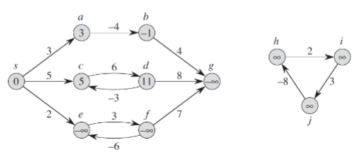
Figure 1
Relaxation
For each vertex v in a graph we maintain an attribute v.d that represents an upper bound on the weight of the shortest path from vertex s to vertex v. v.d is also called shortest-path estimate.
First, we initialize the shortest path estimates and predecessors by following this procedure:
INITIALIZE_SINGLE_SOURCE(G,s)
        for each vertex v in G.V
                v.d = infinity  #estimate
                v.pi = NIL  #predecessor
        s.d = 0
The process of relaxing an edge (u,v) consists of testing if we can improve the shortest path to v found so far by going through u. If so, we update v.d and v.pi.
Why is the term relaxation used to describe an operation that tightens the upper bound? This technique uses inequality v.d < u.d + w(u,v) that compares current value of the shortest path with other possible value for the shortest path. There is no pressure to satisfy this constraint. Thus, there comes name “relaxation.”
The code for relaxation would look as follows:
RELAX(u,v,w)
        if v.d > u.d + w(u,v)
                v.d = u.d + w(u,v)
                v.pi = u
We can see the following examples. In the left example the current estimate for the shortest path to node u is 5 and the current estimate for the shortest path to node v is 9. Now we want to see if we can relax the vertex v going through the vertex u. If we chech the inequelity v.d > u.d + w(u,v) is true since 9 > 5 + 2. Hence, we can update/relax the shortest path to vertex v and assign it a new estimated value of v.d = 7.
Relaxation is widely used. For instance, Dijkstra’s algorithm and the shortest path algorithm for directed acyclic graphs relax each edge exactly once, where Bellman-Ford algorithm relxes each edge |V| - 1 times.
The Bellman-Ford algorithm
Given a weighted graphG =(V,E) with source s and weight function w: E -> R, teh Bellman Ford algorithm returns a boolean value that indicates if the graph contains a negative weight cycle that is reachable from the source vertex s. The algorithm relaxes the edges of the graph until it achieves the actual shortest path with minimum weight. The number of iterations can maximally be |V| - 1. However, that does not mean that relaxation will not reach the minimum weights on 1st or other iteration other than iteration number | v |-1.
BELLMAN-FORD(G,w,s)
        INITIALIZE-SINGLEE-SOURCE(G,s)
        for i =1 to |G.V| - 1
                RELAX(u,v,w)
        for each edge (u,v) in G.E
                if v.d > u.d + w(u,v)
                        return FALSE
        return TRUE
Dijkstra’s Algorithm
Dijkstra’s algorithm solves the single-source shortest-paths problem on a weighted directed graph G = (V,E) for the case in which all edge weights are nonnegative. This algorithm maintains a set S of vertices whose final shortest path weights from the source s have already been determined. The algorithm repeatedly selects a vertex u that is not in the maintainted set S with the minimum shortest path estimate, adds u to the set S, and then relaxes all edges leaving u. What this means is that from the current vertex, the algorithm will select the vertex u with lowest weight. Then it will update any vertex that is connected to the vertex u that can have less value than it has right now (relaxation).
DIJKSTRA(G,w,s)
        INITIALIZE-SINGLEE-SOURCE(G,s)
        S = None
        Q = G.V
        while Q not empty
                u = EXTRACT-MIN(Q)
                S = S union {u}
                for each vertex v in G.adjecant[u]
                        relax(u,v,w)
The Squid